Start Exploring Keyword Ideas
Use Serpstat to find the best keywords for your website


2. What are custom search engines of Google?
2.1 How to create a custom search engine?
3. How to create a Google developer console project?
4. How to retrieve Google search results with every detail into a DataFrame?
5. How to search for multiple queries for multiple locations at the same time for retrieving results into a Data Frame
6. How to refine search queries and use search parameters with Advertools' "serp_goog()" function
6.1 How to use search operators for retrieving SERPs in bulk with Advertools
7. Last thoughts on Holistic SEO and Data Science
Introduction
Python is a programming language that is completely flexible and works within your creativity, in other words, you can set up your own "Keyword Rank Tracker" system with the information you will learn in this article or you can download search results according to different languages and countries at the same time.
First of all, let's start with the custom search engine because you can get a lot of new information in this area.
What are custom search engines of Google?
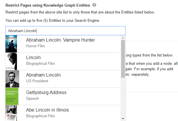
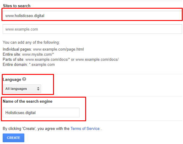
How to create a custom search engine?
However, the topic of this article is about how you can do this by utilizing data science skills and techniques. I will be using Python as the programming language.
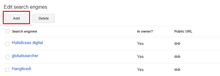
Therefore, you must follow the steps below.
Open the https://cse.google.com/cse/all address.
Click "Add" new for adding a new CSE.
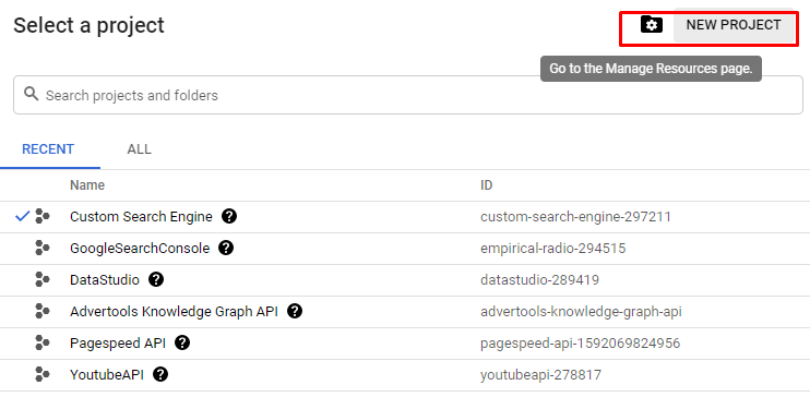
How to create a Google developer console project?
On the Google Developer Console homepage, you will see the "create new project" option. I suggest you give a name that complies with your purpose. In this case, I have chosen the "CSE Advertools" as the name for my project.

How to retrieve Google search results with every detail into a DataFrame?
import advertools as adv
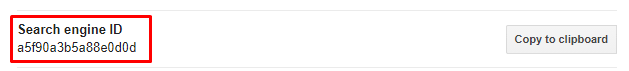
cs_id = "a5f90a3b5a88e0d0d"
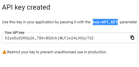
cs_key = "AIzaSyCQhrSpIr8LFRPL6LhFfL9K59Gqr0dhK5c"
adv.serp_goog(q='Holistic SEO', gl=['tr', 'fr'],cr=["countryTR"], cx=cs_id, key=cs_key)At the second line, we have created a variable that stores our custom search engine ID.
At the third line, we have created a variable that stores our custom search API key.
In the fourth line, we have used the "serp_goog()" function with "gl", "cx", "key", "cr" parameters.
Below, you will see our output.
In our first example, we have used the "cr" parameter for only "countryTR" value. It means that we have tried to take only the content that has been hosted on Turkey, or source with a Turkish top level domain. Below, you will see the result differences, when we have removed the "cr" parameter.
df  = adv.serp_goog(q='Holistic SEO', gl=['tr', 'fr'],cr=["countryTR"], cx=cs_id, key=cs_key)
df.shape
We have used the "shape" method on it.
from termcolor import colored
for column20, column40, column60, column90  in zip(df.columns[:20], df.columns[20:40],df.columns[40:60],df.columns[60:90]):
print(colored(f'{column:<12}', "green"), colored(f'{column40:<15}', "yellow"), colored(f'{column60:<32}', "white"),colored(f'{column90:<12}', "red"))I have used a loop with the "zip()" function so that I can use more column segments for the loop.
I have used "for loop" with different variables. I have used "f string" and ">" or "<" signs along with "numbers" that follow them so that I can align the columns and adjust the column's size.
I have used different colors with the color function.
In our first try, we have used two countries within our "gl" parameter. "gl" means "geo-location". We have used "fr" and "tr" values for this parameter which the first one is for France while the latter is for Turkey. And, that's why we have twenty rows.
The first 10 of them is for the "tr" and the last 10 of them is for "fr".
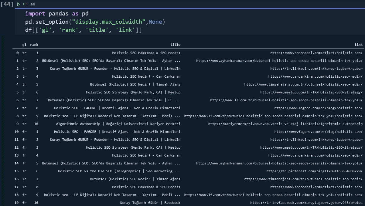
import pandas as pd
pd.set_option("display.max_colwidth",None)
df[['gl', 'rank', 'title', 'link']]
In the second line, I have changed the "Pandas Data Frame" options so that I can see all of the columns with the full length.
I have filtered the specific columns that I want to see.
df_tr = df[df['gl'] == "tr"]
df_fr = df[df['gl'] == 'fr']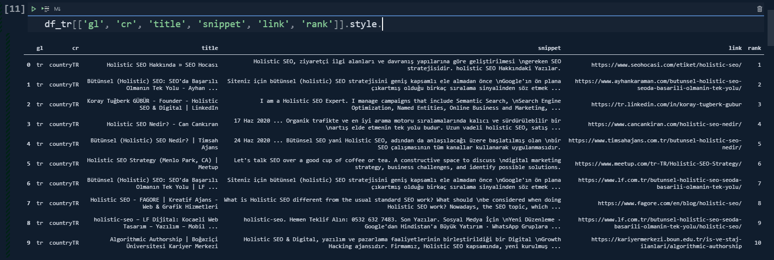
df = adv.serp_goog(q='Who is Abraham Lincoln?', gl=['us'], cr=["countryUS"], cx=cs_id, key=cs_key, start=[1,11,21,31,41,51,61,71,81,91])Dear Elias Dabbas has put a relevant explanation about the "start" parameter and values for a more precise explanation.
By default, the CSE API returns ten values per request, and this can be modified by using the "num" parameter, which can take values in the range [1, 10]. Setting a value(s) for "start", you will get results starting from that value up to "num" more results.
Each result is then combined into a single data frame.
Below you can see the result of the corresponding function call.
But, still, the search engine tries to cover different "possibilities" and "probabilities".
With Advertools' "serp_goog()" function, you can try to see where the dominant search intent shifts and where Google starts to think that you might search for the other kinds of relevant entities or possible search intents.
pd.set_option("display.max_rows",None)
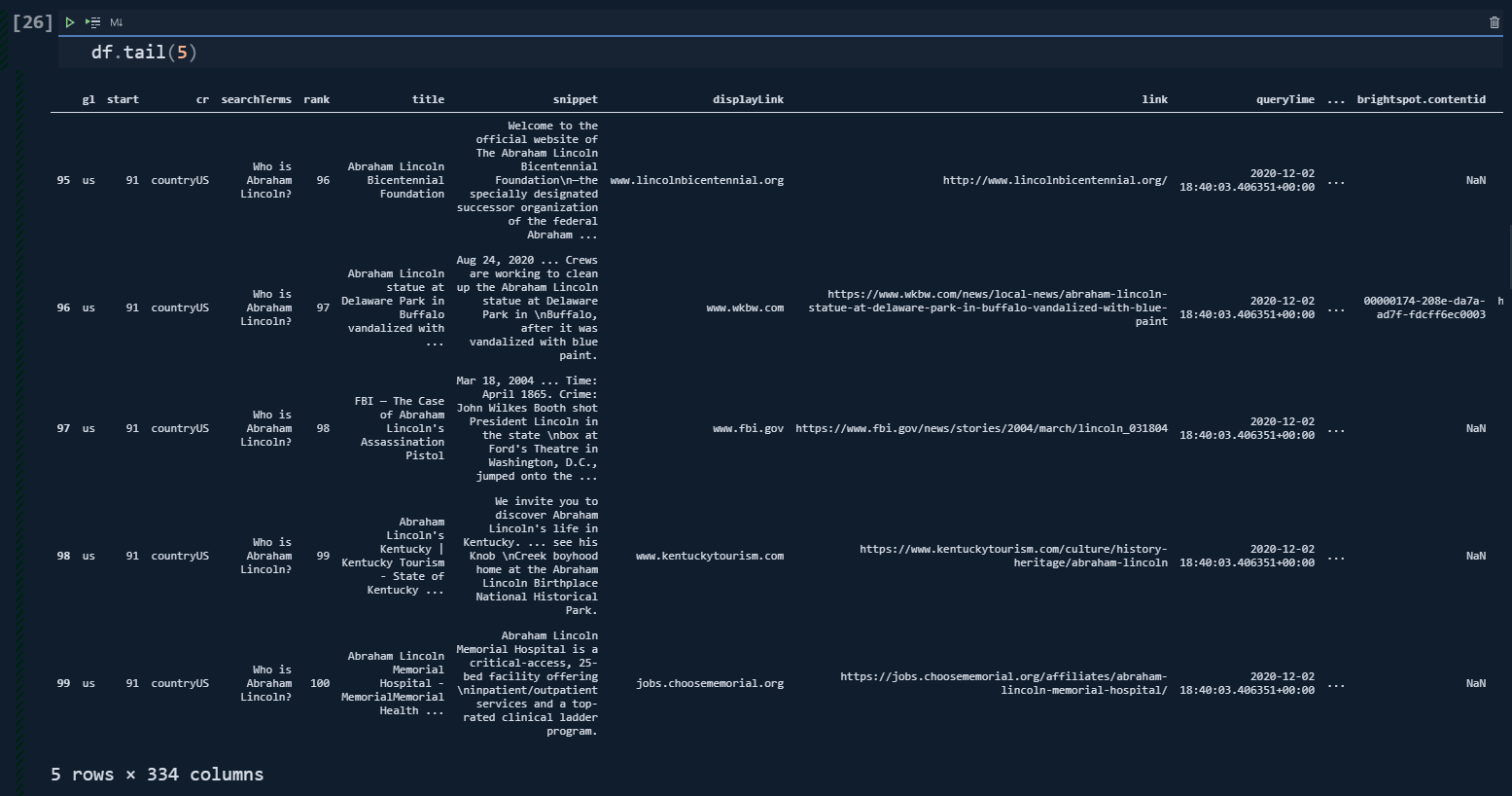
df.head(100)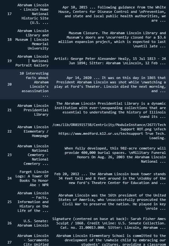
So, only its first paragraph is related to our question, and the content focuses on only a single micro-topic about Abraham Lincoln. You may check the URL below.
https://constitutioncenter.org/blog/10-odd-facts-a...
Or, you can try to search for "Who is Abraham Lincoln" to see what I mean. When we move to the results between 28-38, we see that none of the content is actually relevant to our question.
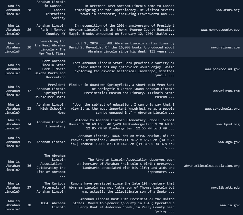
So, with Advertools' "serp_goog()" function, retrieving these intent shifts and intent shifting points, seeing all webpages' angles, differences from each other, side-topics or relevant questions is easy. The best section is that you can do this for multiple queries and combinations of queries and different search parameters, all in one go.
How to search for multiple queries for multiple locations at the same time for retrieving results into a Data Frame
By saying, 15.000 words, I am not joking, I have written a detailed and consolidated article about the Google Knowledge Graph API and Usage of it via Advertools before.
In this article, by respecting Serpstat's editorial guidelines, I will try to cover the most important points in the form of usage style with some important SEO insights. To perform a multi-query search from multi-locations at the same time, you can use the code example below.
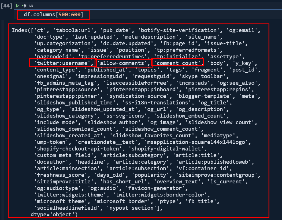
df = adv.serp_goog(q=["Who is Abraham Lincoln?", "Who are the rivals of Abraham Lincoln?", "What did Abraham Lincoln do?", "Was Abraham Lincoln a Freemason"], gl=['us'], cr=["countryUS"], cx=cs_id, key=cs_key, start=[1,11,21,31,41,51,61,71,81,91])Since we have asked 4 questions to Google, and gave 10 start values, 1 "cr", and 1 "gl", we have "4x10x1x1 queries x 10 results" which equals 400. The result pages' features have determined the column count.
You may see the first 100 columns of our results. When we have a unique SERP snippet from a different type, we also have its attributes in the columns such as "postaladdress", "thumbnail", "theme-color", "twitter cards, "application-name" and more.
df[df.docauthor.notna() == True][["docauthor", "htmlTitle", "snippet"]]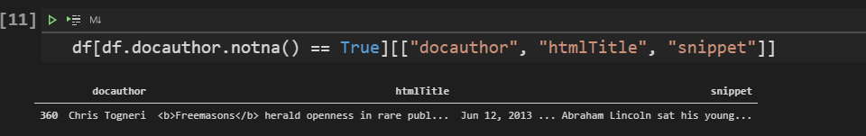
df[df['books:author'].isna() == False][['books:author', "htmlTitle", "snippet"]]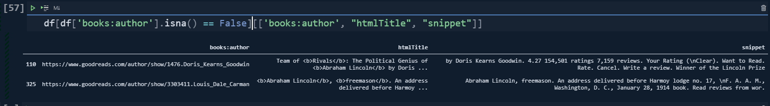
Let's look at them with Advertools.
key = "AIzaSyAPQD4WDYAIkRlPYAdFml3jtUaICW6P9ZE"
adv.knowledge_graph(key=key, query=['Doris Kearns Goodwin', "Louis Dale Carman"])[['result.name', 'result.description', 'resultScore']].style.background_gradient(cmap='Blues')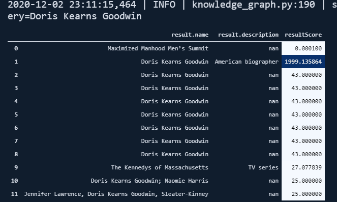
In short:
First, let's learn which domains are top-performing and most-occurred in the Google search results pages for the given four questions.
(df.pivot_table('rank', 'displayLink',
aggfunc=['count', 'mean']).sort_values([('count', 'rank'), ('mean', 'rank')],
ascending=[False, True]).assign(coverage=lambda df: df[('count', 'rank')] / len(df)*10).head(10).style.format({("coverage", ''): "{:.1%}", ('mean', 'rank'): '{:.2f}'})).background_gradient(cmap="viridis")Let's translate the machine language to the human language.
- "df.pivot_table('rank', 'displayLink',) means that you get these two columns to aggregate data according to these.
- "aggfunc=["count","mean"]) means that you get the "count" and "mean" values for these base columns.
- "sort_values([('count', 'rank'), ("mean","rank")]), ascending = [False, True]) means that sort these columns with multiple names with "False" and "True" boolean values. "False" is for the first multi-named column, "True" is for the second one. But, Pandas still shape the entire data frame according to the "count, rank" column since it is superior in order. "Ascending" is for specifying the sorting style.
- "Assign" is for creating new columns with custom calculations.
- "Lambda" is an anonymous function, we are using a column name in "tuple" because in the "pivot_table" every column is a type of multi index, so we are specifying the column with its multi-index values in the tuple.
- "Style.format" is for changing the style of the column's data rows. We are specifying that the column with the name of "coverage, (empty)" should be written with the % sign and with a one "decimal point" while the column with the name of "mean, rank" should be written with two decimal points without a % sign.
- "Background_gradient" is for creating a kind of heatmap for our data frame.
So, in short, machines like to talk less with a systematic syntax than humans.
You may see the result below:
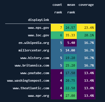
Something wrong in the numbers, top-ranked domains and rank > 10?
On the other hand, we can see that "wikipedia" has the best balance, it has lesser results with a better average ranking.
To see Wikipedia's content URLs, you can use the code below.
df[df['displayLink'] == "en.wikipedia.org"]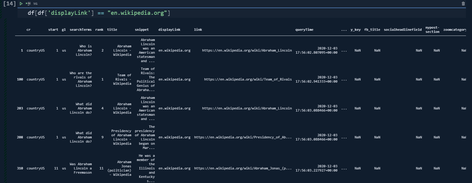
df['displayLink'] = df['displayLink'].str.replace("www.", "")
df_average = df.pivot_table("rank", "displayLink", aggfunc=["count", "mean"]).sort_values([('count', 'rank'), ('mean', 'rank')],
ascending=[False, True])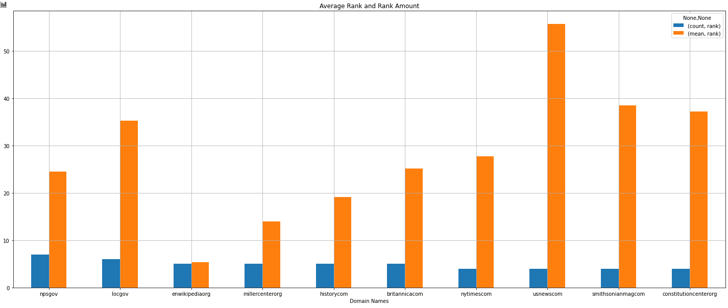
df_average.sort_values(("count", "rank"), ascending=False)[:10].plot(kind="bar", rot=0, figsize=(25,10), fontsize=10, grid=True, xlabel="Domain Names", title="Average Rank and Rank Amount", position=0.5)- We have changed all the "www." values with "" for creating a better and cleaner view for our visualization example.
- We have created a "df_average" variable to create a pivot table based on the "rank" values and "displayLink" data.
- We are using the "aggfunc" parameter so that we can aggregate the relevant data according to the "amount" and "average values".
- With "sort_values" we are sorting the pivot table according to the "count, rank" column as "ascending=False".
- "[:10]" means that it takes only the first ten results.
- "Plot" is the method for the Pandas Library that uses the "matplotlib".
- I have used the "kind="bar" parameter for creating a barplot.
- I have used the "figsize" parameter for determining the figure sizes of the plot.
- I have used a "rot" parameter so that the x axis' ticks can be written as horizontally.
- I have used the "fontsize" parameter to make letters bigger.
- I have used "grid=True" for using a background with grids.
- I have used "xlabel" for determining the X-axis' title.
- And, position parameter to lay the bars more equally is used.
You may see the result below.
You can't plot averages and counts on the same axis.
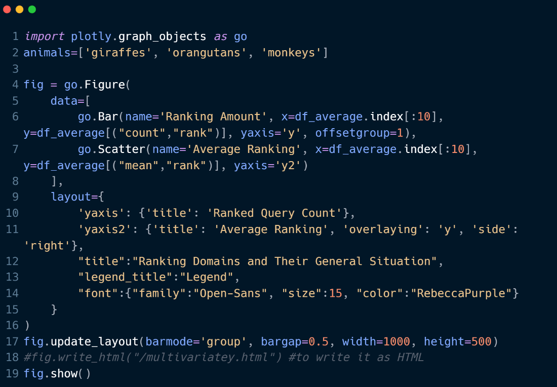
- We have imported, "plotly.graph_objects".
- We have created a figure with a bar and also a scatter plot with the "go.Figure(data)".
- We have used a common X Axis Value which is our "df_average" dataframe's indexes which is equal to the most successful domains for our example queries.
- We have arranged the plot's "y axis" and "x axis" names, values, fonts, sizes with the "layout" parameter.
- We have adjusted the width and height values with "update_layout" for our plot and called it with "fig.show()".
- If you want to write it into an HTML file, you can also use the "fig.write_html" function that I have commented out.
Below, you will see the output.
We see that Wikipedia, Britannica, Millercenter, and History.com have better rankings averagely, and also "Nps.gov" and "Loc.gov" have more results for these queries, and their average ranking is close to Britannica.
Perform the same progress for multiple queries. You will get your Ranking Tracker for sure. You can schedule a function or code block the run repeatedly per specific timelines with Python's Schedule Library, but this is a topic of another article.
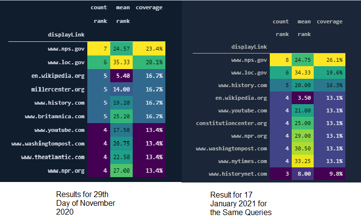
Before moving further, let me show you the same SERP Record after Google's Broad Core Algorithm Update on 3rd December of 2020.
Let's perform another visualization and see which domain was at which rank before the Core Algorithm Update and how their rankings affected.
You may see our machine command below.
import matplotlib.pyplot as plt
from matplotlib.cm import tab10
from matplotlib.ticker import EngFormatter
queries = ["Who is Abraham Lincoln?", "Who are the rivals of Abraham Lincoln?", "What did Abraham Lincoln do?", "Was Abraham Lincoln a Freemason"]
fig, ax = plt.subplots(4,1, facecolor='#eeeeee')
fig.set_size_inches(10, 10)
for i in range(4):
ax[i].set_frame_on(False)
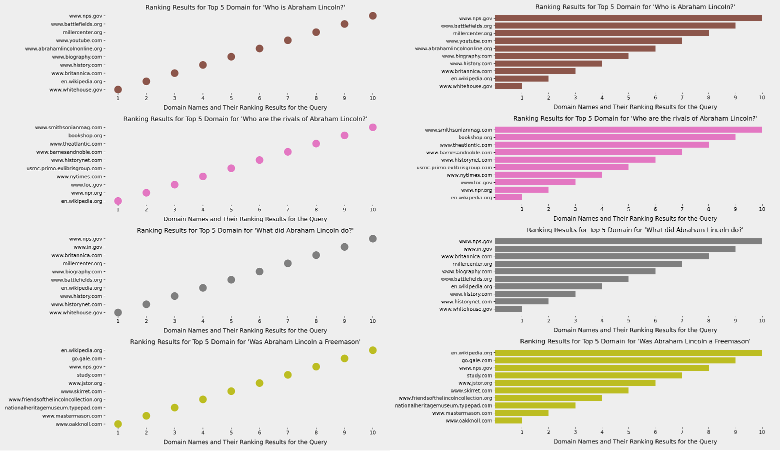
ax[i].barh((df[df['searchTerms']==queries[i]])['displayLink'][:5], df[df['searchTerms']== queries[i]]['rank'][:5],color=tab10.colors[i+5])
ax[i].set_title('Ranking Results for Top 5 Domain for ' + "'" + queries[i] + "'", fontsize=15)
ax[i].tick_params(labelsize=12)
ax[i].xaxis.set_major_formatter(EngFormatter())
plt.tight_layout()
fig.savefig(fname=”serp.png”, dpi=300, quality=100)
plt.show()- We have imported Matplotlib Pyplot, "tab10" and "EngFormatter". The first one is for creating the plot, the second one is for changing the colors of the graphics and the last one is for formatting the numbers as "5k, 6k" instead of 5000, 6000 in the graphs.
- We have created a list from our "queries" with the name of "queries".
- We have created two different variables which are fig, ax and we have assigned "plt.subplots" function's result to them.
- We have created a subplot with four rows and changed the "facecolor" of it.
- We have changed the figure size with the "set_size_inches".
- And, for every query we have chosen, we have started a for loop to put them into our figure with multiple plots.
- We have used "barh" method to create horizontal bars.
- We have used Pandas Methods to match the "query" and "search term" for filtering our related rows.
- We have changed every plot's color with the "tab10.colors" within the "color" parameter.
- We have changed the title of every plot with the name of the matching query.
- We have changed font sizes with the parameter "fontsize".
- We have used "labelsize" with the "tick_params" method to change the size of the tick parameters.
- We formatted the xticks so that the relevant data can be displayed more clearly. "EngFormatter ()", which is used to display xticks in different "units of measure" on different subjects, may not work properly at this point as we use very few "queries".
- We have used a tight layout with the "tight_layout()".
- We have saved our figure into an image with png extension with the "300 DPI" and "maximum resolution" quality.
- We have called our figure.
And, you may see the result below. This is the result after the Core Algorithm Update.
Thus, using "plotly.graph_objects" with a for loop and line chart can help fix this issue better.
fig.data = []
fig = go.Figure()
for i, domain in enumerate(df_graph_first_10["Domain"]):
filtered_graph = df_graph_first_10[df_graph_first_10["Domain"]==domain]
fig.add_scatter(x=filtered_graph["Query"], y=filtered_graph["Rank"], name=domain, text=[filtered_graph["Domain"]])
fig.update_layout(width=1400, height=800, legend=dict(
yanchor="top",
y=1.5,
xanchor="right",
x=1.3),
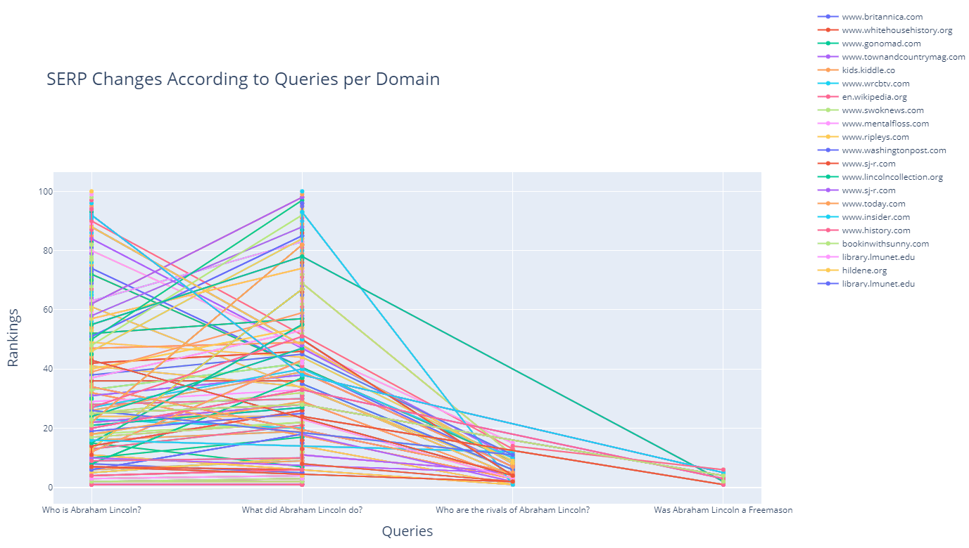
hovermode="x unified", title="SERP Changes According to Queries per Domain", title_font_family="Open Sans", title_font_size=25)
fig.update_xaxes(title="Queries", title_font={"size":20, "family":"Open Sans"})
fig.update_yaxes(title="Rankings", title_font={"size":20, "family":"Open Sans"})
fig.write_html("serp-check.html")
fig.show()- fig.data=[] is for clearing the figure.
- go.Figure() is for creating the figure.
- "name" and "text" parameters are for determining the name of the traces and text for the hover.
- In the "fig.update_layout()", we are determining the title, title font, legend, and legend position.
- We ar eusing "fig.update_xaxes" and "fig.update_yaxes" for determining the axes titles and font styles.
- We also used "write_html" for saving the plot into an HTML file.
- We also used "unified x" as the hover mode.
As a line, you can see how a domain's ranking changes for which query in an interactive way as below.
(df.to_csv("df_after_core_algorithm_update.csv")
How to refine search queries and use search parameters with Advertools' "serp_goog()" function
Before finishing this small guideline, I wanted to show also how to use Search Parameters with the "serp_goog()" function of Advertools. With Advertools, we can use Google search operators with the help of custom Search API Parameters to understand and explore Google's algorithms and SERP's nature. Thanks to search parameters, you can try to understand Google's algorithm in a better and detailed way for different types of queries and also topics. Below, you will find an example.
df = adv.serp_goog(q=["Who is Abraham Lincoln?", "Who are the rivals of Abraham Lincoln?", "What did Abraham Lincoln do?", "Was Abraham Lincoln a Freemason"], gl=['us'], cr=["countryUS"], cx=cs_id, key=cs_key, start=[1,11,21,31,41,51,61,71,81,91], dateRestrict='w5', exactTerms="Mary Todd Lincoln", excludeTerms="kill", hq=["the president","childhood"])- "dateRestrict" is for only showing the results and their documents that are created in the last five weeks.
- "exactTerms" are for filtering the documents that include the term that we specified.
- "excludeTerms" are for excluding the documents that include the term that we specified.
- "Hq" is for appending the different terms to the queries we have chosen.
In this example, I have chosen to extract only the documents that have been produced in the last 5 weeks, and include the "Mary Todd Lincoln" who is the wife of Abraham Lincoln, and exclude the term "kill" while appending the "the president" and "childhood" terms to my query group.
What was my angle here? I have tried to extract the latest and updated documents that focus more on Abraham Lincoln's true personality and his family, including his "administration" and also "family life" without the term "kill."
The lesson here is that you can specify different types of query patterns and entity attributes and entity-seeking queries to see which types of content rank higher for which types of entities and their related queries.
For instance, Google might choose to rank higher documents that include Abraham Lincoln's wife's name and her entity attributes along with his administration instead of web pages that solely focus on the assassination. And, now you might see how the results change as below.
df_graph_10 = df_graph[df_graph["Rank"]<=10]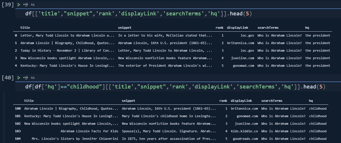
Until now, we have seen the search and query refinement with Python for retrieving the SERP. Lastly, we will cover the major search operators.
How to use search operators for retrieving SERPs in bulk with Advertools
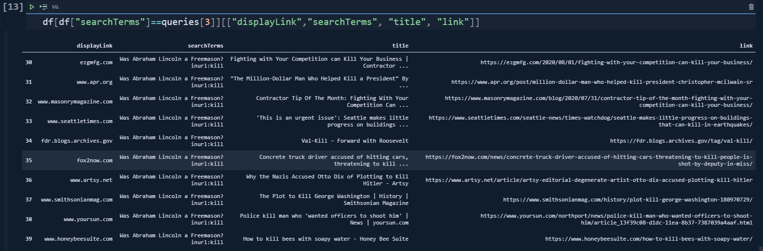
queries = ["Who is Abraham Lincoln? site:wikipedia.org", "Who are the rivals of Abraham Lincoln? -wikipedia.org", "What did Abraham Lincoln do? intitle:President", "Was Abraham Lincoln a Freemason inurl:kill"]
df = adv.serp_goog(q="Who killed Abraham Lincoln site:wikipedia.org", cx=cs_id, key=cs_key)In the first query, we have requested only the results from "wikipedia.org".
df[df["searchTerms"]==queries[0]]["displayLink"].str.contains("wikipedia")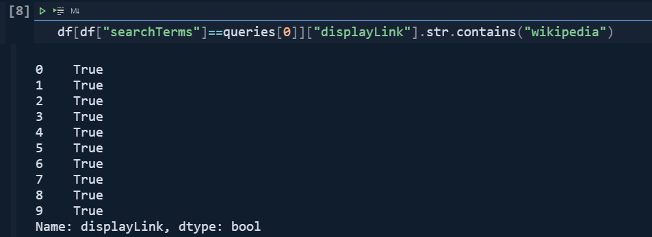
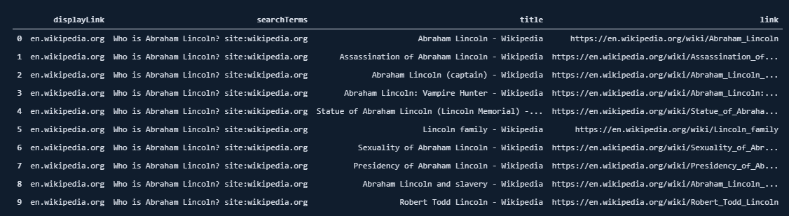
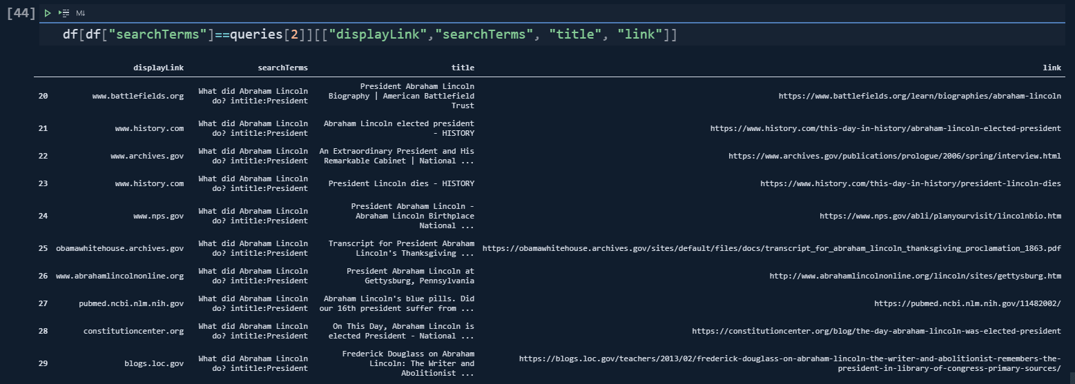
df[df["searchTerms"]==queries[0]][["displayLink","searchTerms", "title", "link"]]
df[df["searchTerms"]==queries[1]]["displayLink"].str.contains("wikipedia")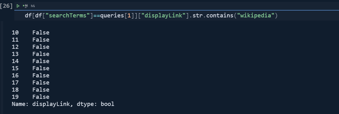
df[df["searchTerms"]==queries[1]][["displayLink","searchTerms", "title", "link"]]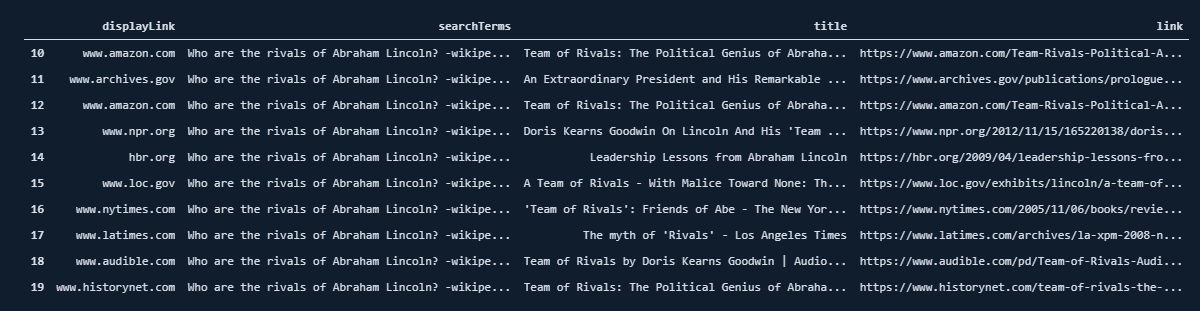
df[df["searchTerms"]==queries[2]]["title"].str.contains("President", case=False)
df[df["searchTerms"]==queries[3]]["link"].str.contains("kill", case=False)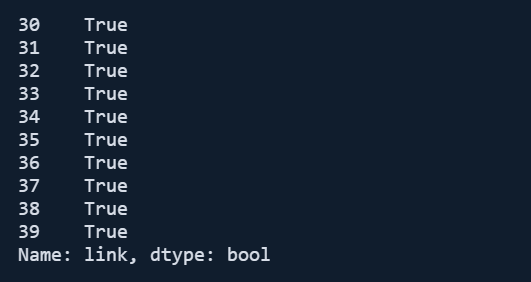
So, there are lots of different result characters for the same query and search intent, to satisfy the search engine, examining all these results for the same entity groups with the same query types, excluding and including terms or using "links," "n-gram analysis," "structured data" and more is going to help SEOs to see how to rank at to the first rank with the help of Data Science.
Last thoughts on holistic SEO and data science
And, Data with Intelligence is your best alliance for this purpose. You can understand the algorithms of search engines with data and your intelligence. And, Holistic SEO is just an acronym for coding and marketing intersection, in my vision.
Speed up your search marketing growth with Serpstat!
Keyword and backlink opportunities, competitors' online strategy, daily rankings and SEO-related issues.
A pack of tools for reducing your time on SEO tasks.
Discover More SEO Tools
Backlink Cheсker
Backlinks checking for any site. Increase the power of your backlink profile
API for SEO
Search big data and get results using SEO API
Competitor Website Analytics
Complete analysis of competitors' websites for SEO and PPC
Keyword Rank Checker
Google Keyword Rankings Checker - gain valuable insights into your website's search engine rankings
Recommended posts
Cases, life hacks, researches, and useful articles
Don’t you have time to follow the news? No worries! Our editor will choose articles that will definitely help you with your work. Join our cozy community :)
By clicking the button, you agree to our privacy policy.